System Approach to the Migration

Introduction:

Akin L. Mabogunje is an African Scholar who has approached rural-urban migration from different point of view rather than prevailing approaches.It shows the system approach to rural-urban migration is concerned not only with why people migrate but also with the implications and consequences of the process. This theory is designed to answer why and how a rural individual become a permanent city dweller as well as what factors are operating on the

system. This theory is written with the particular reference to Africa.

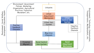
1.     Environment:

Comprises “the set of all objects a change in whose attributes affects the system, and also those objects whose attributes are changed by the behaviour of the system. This is the environment which stimulates the villager to desire change in the basic locale and rationale of his economic activities and which, in consequence, determines the volume, characteristics, and importance of rural-urban migration.

2. System:

A system may be defined as a complex of interacting elements, together with their attributes and relationships . Figure  indicates the basic elements in the rural-urban migration system as well as the environment within which the system operates. It identified first the potential migrant who is being encouraged to migrate from the environment.

3. Sub-System:

. A control sub-system is one which oversees the operation of the general system and determines when and how to increase or decrease the amount of flow in the system.There are two types of sub-system:

        I.             Rural Sub-System: family structure,age at marriage, age at economic independent, land tuner or holding system,agriculture activities,etc.

     II.             Urban Sub-System: employment opportunities, residential facilities, urban wages,etc.

 The urban control sub-system operates at the opposite end of the migrant’s trajectory to encourage or discourage them from being absorbed into the urban environment. Absorption at this level is of two kinds:

1.     Residential

2.     Occupational

4. Adjustment Mechanism:

•       These are the series of factors in the environment which acts like push or pull factors and operates both the rural and urban sub-system. It is also of two types:

1.     Rural Adjustment Mechanism : agriculture production, types of production, income, land tenure system, land distribution and ownership

2.      Urban Adjustment Mechanism: socio-economic needs of migrants, own community, ethnic union

 Urban adjustment mechanism act both positively or negatively to adjust migrant in the urban sector.

5.Energy:

A system comprises not only matter (the migrant, the institutions,and the various organizations mentioned) but also energy. In the physical sense, energy is the capacity of body to do work. It can be expressed  two forms of it which are relevant here :“potential energy’’ which is the body’s power of doing work by virtue of stresses resulting from its relation either with its environment or with other bodies and the second form is “kinetic energy” which is the capacity of a body to do work by virtue of its own motion or activity. In a theory of rural-urban migration:

1. Potential energy can be likened to the stimuli acting on the rural individual to move.

2. Kinetic Energy is translation of potential energy when the individual has been successfully dislodge from the rural area.

Relationship between the System and Environment:

Systems can be classified into three categories depending on the relationship they maintain with their environment;

1. Isolated systems which exchange neither “matter” nor “energy” with their

Environment

2. Closed systems which exchange “energy” but not “matter”;

3. Open systems which exchange both “energy” and “matter”

Zipf's Inverse Distance Law

Introduction:

G.K Zipf, a well known geographer developed the gravity hypothesis of migration based on Ravenstein laws of migration ;most of the migrants are from short distance and igration proceeds step-by-step. It is also known as (P1 X P2)D hypothesis or social physics of Newton.It is used to predict the interaction between two places.This law is based Newtons Gravitational Law which states that gravitational force between two bodies is directly proportional to the product of their masses and

inversely proportional to the distance between them.This model can be use to explain :

1.      Traffic Flow

2.      Migration between two areas

3.      The number of people likely to use one central place.

Statement of the Law:

There is an inverse relationship between the numbers of people moving and the distance moved. The volume of migration between the two places, (mainly place of origin and place of destination) is directly proportional to the size of two places and inversely proportional to the distance between the places.

Mathematically:

Iij=k . Pi.Pj/Dij

Where, Iij=Volume of migration from i to j

            Pi and Pj=Size of place i and j in-terms of area, population, socio-economic  setting                     

            Dij=Distance between i and J

              K=a constant

            

Explanation of the Figure:

•      The gravity is the force of attraction of earth pulls an object towards its center or surface. In this hypothesis, the gravity is symbolized to show the forces that pull the people towards the place of destination.In this model, according to Zipf, people will migrate even if they are not pushed from their place of origin, they migrate because they are pulled by better socio-economic future at the some other place (destination). In the gravity, earth pulls any objects towards it surface, in a similar way ; people are pulled towards the big cities by its pull effect (same as gravity) not by push effect at the place of origin.  This attraction force is determined by the size of destination in-terms of socio-economic facilities, size of population and distance between place of origin and destination. In this model, the pull factors are treated as ‘attracting mass’ and while the mass pull , the distance acts as friction to migration.

 

Bongaart's Proximate Determinats Of Fertility

In the year 1970, Bongaart refined the Davis and Blake's eleven intermediate variables of fertility into nine direct determinants of fertility called 'proximate determinats of fertility '. According to the Bongaarts, " the proximate determinants of fertility are the biological and behavioral factors through which social, economic and environmental 

variables affects fertility ".

The proximate determinants of fertility can be classified in two groups: 

1) Proximate Determinats Influencing Length of Reproductive Span

2) Proximate Determinats Influencing the rate of child-bearing within the Reproductive Span.

1) Proximate Determinats Influencing Length of Reproductive Span 

It includes the time period between first menstruation/ menarche and menopause. The menarche marks the beginning of the reproductive span or period and menopause marks the end of the reproductive period. It also includes marriage, divorce and separation, windowhood etc. which may have positive or negative impact in fertility. 

2) Proximate Determinats Influencing the rate of child bearing within the Reproductive Span 

Within the reproductive span, the married and fecund women reproduce at a rate inversely related to the average duration of the birth interval. Higher fertility is associated with short birth interval and lower fertility is associated with long birth intervals. The duration or length of her birth interval is determined by following components: 

1) Post-Partum infecundable period 

2) Conception Wait

3) Gestation period 

The above component of birth interval can be shown in the following diagram: 

a. Birth Interval without Intrauterine Death

b. Time Added by Intrauterine Death

1) The Post-Partum Infecundable Period

After the child-birth, a women passes through an infecundable period during which the normal pattern of ovulation and menstruation is absent, this is called Post-Partum infecundable period. The length of Post-Partum Infecundable period is primarily determined by the length of breastfeeding. With the increase in the duration of breastfeeding, the length of the amenorrhea period also increases which inturn increases the Post-Partum amenorrhea period. 

2) The waiting time to Conception 

This period which is also known as fecundable or ovulatory interval comprises the period from onset of ovulation after child-birth to conception. The length of this interval is determined by  natural fecundability and the use and effectiveness of contraception. Where  natural fertility is high and no use of contraceptive method is made the period of conception wait shorter. This period is lengthened with declining natural fertility and with higher practice and effectiveness of conception. 

3) Gestation period 

The period of full-term pregnancy doesnot vary much and its duration is assumed to be nine months. However, in case of pregnancy ends prematurely in a spontaneous or induced intrauterine death, the duration of the birth internal is lengthened by the additional components as plane B in the above figure.

Thus it is observed that the seven proximate determinants are:

1.Marriage

2. Onset of permanent sterility

3. Post-Partum in-fecundability 

4. Natural fecundability or frequency of intercourse

5. Use and effectiveness of contraception 

6. Spontaneous intrauterine mortality; and 

7. Induced abortion

 It is clear that the first two of these seven determinants determine the length of reproductive span and the other five determine the rate of child-bearing.

Ravenstein Laws of Migration:

Introduction:

Ernst George Ravenstein was a British statistician who wrote two articles and published a paper entitled “The Laws of Migration” in 1885 which is based on the data related to migration between England and Wales in the 1880s decade. He argued that migration was not random but governed by general laws and this law was effected by variables such as distance, transportation, motive, etc. In his first thesis, he put forward the general laws of migration which concentrate to the internal migration, whereas second

is based onthe international migration.

Laws of Migration:

Law 1: Most of the migrants are from short-distance.

There is inverse relationship between the distance and the number of migrants(volume of migration). If there is short distance between the place of origin and destination, the volume of migration will be high compare to the longer distance. So, the majority of migrants go only short distance.

Law 2: Migration proceeds step by step.

Inhabitants of remote area tend to migrate towards the small town then after the larger city. Most of the people are not able to migrate directly towards the big cities from the rural areas.

Law 3: Each migration current produces a compensating counter-current.

The volume of migration stream is larger than the counter-stream. If we observe the trend of Nepalese migration, the flow of migration from Hill and Mountain to Terai and its counter-stream is from Terai to Hill and Mountain. Where, the volume of migration from Hill to Terai is much larger than its counter-stream.

Law 4: Most of the migrants are rural born

Urban born people are less migratory than the people in rural areas. Most of the people migrate for the betterment of their living and to acquire amenities. The urban natives are already utilizing the urban facilities ,so there is not necessary to migrate. But rural natives are deprived from facilities such as education ,health , transportation , communication and employment , so people migrate from remote area to urban area.

Law 5: Females are more migratory than males in short distance.

The volume of female migration is higher than the male in short distance as well as internal migration only. This is due to the marriage causes. Whereas, male are more common in international migration and cover long distance compared to the female.

Law 6: Migration increases with the improvement in technology.

The advancement of technology creates job opportunities as well as facilities for better livelihood .So, the size of migration increases with the development .

 

Law 7: There is always a motive behind migration especially economic motive

There is motive behind migration where as economic motive have primacy among the various factors governing magnitude of migration. Motive refer to the employment , education and better earning.

 

 

 

Intermediate Variable Framework Of Davis and Blake

Davis and Blake (1956)3 identified a set of 11 'intermediate variables' which directly affect fertility which they grouped into the following three categories. Bongaarts (1978) further refined the list of proximate determinants.

Factors Affecting Intercourse Variables

A. Those governing the formation and dissolution of unions in the reproductive period

1. Age of entry into sexual unions
2. Permanent celibacy: proportions of women never entering sexual unions
3. Amount of reproductive period spent after or between unions
   1. When unions are broken by divorce, separation, or desertion
   2. When union are broken by death of husband

B. Those governing the exposure to intercourse within union

4. Voluntary abstinence
5. Involuntary abstinence (from impotence, illness, unavoidable but temporary separations)
6. Coital frequency (excluding periods of abstinence)

Factors Affecting Conception Variables

7. Fecundity or infecundity, as affected by involuntary causes
8. Use or non-use of contraception
9. Fecundity or infecundity, as affected by voluntary causes

Factors Affecting Gestation Variables

10. Foetal mortality from involuntary causes
11. Foetal mortality from voluntary causes

In the process of child bearing three stages may be easily identified:

1) Intercourse

2)Conception 

Business Cycle

Definition:

It refers to the fluctuations in output and employment with alternating periods of time. It shows a rise or fall in aggregate output, national income and employment in the economy.

Features of Business Cycle:

1. It is periodic and regular which means it operates at regular interval of 10 to 12 years and all the phases came regularly.

2. It covers all the sectors.

3.

It is universal which means it is found in every countries.

4. It is self-reinforcing.

Phases of Business Cycle:

1. Expansion:

In the expansion phase, there is an increase in various economic factors, such as production, employment, output, wages, profits, demand and supply of products, and sales. The prices of factor of production and output increases simultaneously. In this phase, debtors are generally in good financial condition to repay their debts; therefore, creditors lend money at higher interest rates. This leads to an increase in the flow of money.

In expansion phase, due to increase in investment opportunities, idle funds of organizations or individuals are utilized for various investment purposes. Therefore, in such a case, the cash inflow and outflow of businesses are equal. This expansion continues till the economic conditions are favorable.

2. Peak:

The growth in the expansion phase eventually slows down and reaches to its peak. This phase is known as peak phase. In other words, peak phase refers to the phase in which the increase in growth rate of business cycle achieves its maximum limit. In peak phase, the economic factors, such as production, profit, sales, and employment, are higher, but do not increase further. In peak phase, there is a gradual decrease in the demand of various products due to increase in the prices of input.

The increase in the prices of input leads to an increase in the prices of final products, while the income of individuals remains constant. This also leads consumers to restructure their monthly budget. As a result, the demand for products, such as jewellery, homes, automobiles, refrigerators and other durables, starts falling.

3. Recession:

As discussed earlier, in peak phase, there is a gradual decrease in the demand of various products due to increase in the prices of input. When the decline in the demand of products becomes rapid and steady, the recession phase takes place.

In recession phase, all the economic factors, such as production, prices, saving and investment, starts decreasing. Generally, producers are unaware of decrease in the demand of products and they continue to produce goods and services. In such a case, the supply of products exceeds the demand.

Over the time, producers realize the surplus of supply when the cost of manufacturing of a product is more than profit generated. This condition firstly experienced by few industries and slowly spread to all industries.

This situation is firstly considered as a small fluctuation in the market, but as the problem exists for a longer duration, producers start noticing it. Consequently, producers avoid any type of further investment in factor of production, such as labor, machinery, and furniture. This leads to the reduction in the prices of factor, which results in the decline of demand of inputs as well as output.

4. Trough:

During the trough phase, the economic activities of a country decline below the normal level. In this phase, the growth rate of an economy becomes negative. In addition, in trough phase, there is a rapid decline in national income and expenditure.

In this phase, it becomes difficult for debtors to pay off their debts. As a result, the rate of interest decreases; therefore, banks do not prefer to lend money. Consequently, banks face the situation of increase in their cash balances.

Apart from this, the level of economic output of a country becomes low and unemployment becomes high. In addition, in trough phase, investors do not invest in stock markets. In trough phase, many weak organizations leave industries or rather dissolve. At this point, an economy reaches to the lowest level of shrinking.

5. Recovery:

As discussed above, in trough phase, an economy reaches to the lowest level of shrinking. This lowest level is the limit to which an economy shrinks. Once the economy touches the lowest level, it happens to be the end of negativism and beginning of positivism.

This leads to reversal of the process of business cycle. As a result, individuals and organizations start developing a positive attitude toward the various economic factors, such as investment, employment, and production. This process of reversal starts from the labor market.

Consequently, organizations discontinue laying off individuals and start hiring but in limited number. At this stage, wages provided by organizations to individuals is less as compared to their skills and abilities. This marks the beginning of the recovery phase.

In recovery phase, consumers increase their rate of consumption, as they assume that there would be no further reduction in the prices of products. As a result, the demand for consumer products increases.

In addition in recovery phase, bankers start utilizing their accumulated cash balances by declining the lending rate and increasing investment in various securities and bonds. Similarly, adopting a positive approach other private investors also start investing in the stock market As a result, security prices increase and rate of interest decreases.

Price mechanism plays a very important role in the recovery phase of economy. As discussed earlier, during recession the rate at which the price of factor of production falls is greater than the rate of reduction in the prices of final products.

Therefore producers are always able to earn a certain amount of profit, which increases at trough stage. The increase in profit also continues in the recovery phase. Apart from this, in recovery phase, some of the depreciated capital goods are replaced by producers and some are maintained by them. As a result, investment and employment by organizations increases. As this process gains momentum an economy again enters into the phase of expansion. Thus, a business cycle gets completed.

Some Parts are Adopted from: https://www.economicsdiscussion.net/business-cycles/5-phases-of-a-business-cycle-with-diagram/4121



 

 

 

 

 

 

 

Saving, Saving Function, Average Propensity to Save and Marginal Propensity to Save

Saving is defined as the excess of income over consumption expenditure. The concept of saving is closely related to the concept of consumption. Saving is the part of income that is not consumed. Generally, as the level of income increase, saving also increases and vice versa.

Saving function or the propensity to save expresses the relationship between saving and the level of income. It is simply the desire of the households to hoard a part of their total disposable income.

Symbolically, the functional relation between saving and income can be defined as S= f(Y).

We know,

Y= C + S;

Thus, S= Y-C;

Where, Y= Income; S= Saving; C= Consumption

The equation shows that the remaining amount after the deduction of total expenditure from total income is saving. Thus, saving is that part of income which is not spent on consumption

---

Relationship between Saving and Income

• A direct relationship exists between saving and income. This means, if income increases, saving also increases but in less proportion in comparison to income.
• When income level is low, saving is negative. In the initial stages when income is low, consumption expenditure is more than in comparison to the level of earning, so there is no saving .i.e. dis-saving.

The table and diagram below clearly explains the relationship between income and saving:

Income (Y)	Consumption (C)	Saving (S)	APS (S/Y)	MPS (ΔS/ ΔY)
0	20	-20	–	–
60	70	-10	–	–
120	120	0	0	–
180	170	10	0.06	0.17
240	220	20	0.08	0.17

---

Attributes of Saving Function

Saving function or propensity to save has two major attributes:

• Average Propensity to Save (APS)
• Marginal Propensity to Save (MPS)

Average Propensity to Save (APS)

The average propensity to save is a relationship between total saving and total income in a given period of time. It is the ratio of saving to income that shows the portion of the income that people saved.

Symbolically,

APS=S/Y

Where, S= Saving; Y= Income

For example, when the disposable income is 180, consumption is 170, and saving is 10, we can calculate APS as

APS= 10/180 =0.06 or 6%

This shows that out of total income in a year, 6 % will be saved after spending on consumption. As shown in the table above, we can see that the average propensity in save increases with the increase in income .i.e. APS increased from 0.06 to 0.08 with the increase in income.

Diagrammatically,

APS is a point on the curve S, and it is measured as S₁Y₁/OY₁.

Marginal Propensity to Save (MPS)

The marginal propensity to save or MPS refers to the increase in the proportion of saving as a result of increase in the level of income. It can be defined as the ratio of change in saving to change in income.

Symbolically,

MPS=ΔS/ΔY

Where, ΔS= Change in saving; ΔY= Change in income

For example, when income increased from 180 to 240, savings also changed from 10 to 20. We can then calculate MPS as

MPS= 10/60 =0.17 or 17%

This shows that, when income increased, the proportion of saving also increased. The saving made out of total income is 17%.

Diagrammatically,

In the diagram, BC is the change in income and AB is the consequent change in saving. So, MPS is AB/BC.

---

Determinants of Saving Function

The determining factors that contribute to the saving function include Desire to save, Power to save, and Facilities to save.

Desire to Save

The desire or the willingness of an individual or household to save is the major driving factor towards saving. The factors that affect the desire of an individual to save are

i. Level of income

Level of income is an important determinant of saving in any economy or country. Higher the level of income for any household or individual, higher the level of saving.

ii. Provisions for the future

The future requirements of money is uncertain. So, in order to have a secured future against any uncertain events, saving up at present helps to have a pool of extra money. Savings can be taken as a precaution for any unforeseen needs in the future.

---

Ability to Save

In spite of the willingness to save, one cannot save if they do not have the capacity or the ability to save. Saving is only possible if an individual can meet all their consumption expenditures and still save up, then it can be said that they have the ability to save. Ability to save depends on the level of income and consumption expenditure.

The factors that determine the ability to save include

i. Labor Efficiency

The ability or power to save depends on the efficiency of labor. If an economy has an efficient group of people, it increases production efficiency as well. This results in increasing income and thus people can have more money that can be saved, even after meeting the consumption expenditures.

ii. Size of National Income

Higher the national income, greater is the ability to save. Low national income in developing and under-developed countries is the main reason for no saving being made.

iii. Developmental activities

The development of various sectors like trade, industrial areas, agricultural sector, etc. is a source of increased income level, as there will be more inflow of money into the economy.

---

Facilities to Save

Saving also depends on the facilities availability. This includes:

i. Development of financial institutions

The development and expansion of financial institutions like banks, co-operatives, etc. encourage people to save more with their effective marketing strategies. They also provide attractive interest rates on savings.

ii. Rate of interest

Attractive interest rates encourage people to save more. When the interest rates are high in the market, people save more, and when the rates are low, they withdraw and spend on consumption.

iii. Social security system

The provision of security system such as old age pensions, medical insurance, unemployment allowance, etc. reduces the rate of saving in a country. When there is adequate provision of social security in the society, people feel secured about their future and they spend more of their income on consumption.

iv. Taxation Policy

Progressive taxes reduce saving as taxes increase with the increase in income. People with higher income save less because of the taxes they need to pay. But if the taxes on expenditure are higher then, they are encouraged to spend less and save more.

v. Fiscal policy

The fiscal policy of the government affects the level of saving in a country. If taxes are imposed on necessary commodities, people cannot save more. The reduction of taxes on basic goods leads to an increase in the level of saving. Also, if taxes are high on luxury goods, people are enticed to save more than to purchase luxury goods. 

Adopted from: https://www.businesstopia.net/economics/macro/saving-function

Causes and Effects of Inflation

Causes of Inflation:

a. Demand Pull Inflation

Inflation caused due to excessive demand is termed as demand pull inflation. It exists in the economy when overall price of goods and services increase due to increase in aggregate demand, but the 

aggregate supply remains the same.

When the economy is at full employment, it is not possible to produce goods and services any further because the available resources have been optimally utilized. In this case, the supply of commodities is limited, but the demand is increasing. Consequently, the price of the commodity rise and leads to

Inflation and its Measurement

Inflation

It is the situation of continuous increase in price of the goods and services during which the quantity of money increases but the value of money decreases.

Important Characteristics of 

Inflation:

1. It is regular and continuous.

2. It is cumulative.

3. It is the situation of the increase in general price level not the increase in individual price.

4. The supply of goods and services is less in comparison to their demand.

Measurement of Inflation:

Inflation is measured in percentage which is obtained by calculating the change in percentage of current price index over the previous one. The price index is developed by carrying out a survey on the basis of actual survey on market prices of various goods and services. These goods and services are put together into ‘market basket’. The cost of identical market basket today is compared to the cost of identical basket in the previous year or a base year in order to determine the rate of inflation.

---

1. Consumer Price Index (CPI)

It is an measure of inflation which measures changes in price from the purchasers’ perspective. It is a measure of price changes in consumer goods and services such as food, clothing, gasoline and automobiles but excludes housing costs and mortgage interest payments. It reflects changes in the prices of a market basket of goods and services purchased by consumers (individuals and households). CPI helps in the measurement of cost of living of urban consumers.

CPI is a statistical estimate constructed with the help of prices of items that represent the economy, whose prices are collected periodically. The annual percentage change in CPI is taken as a measure of inflation.

Thus,

Where,

CPI₁ = CPI in previous year

CPI₂ = CPI in current year

Calculating CPI

Calculation of CPI and inflation requires data on prices of goods and services in large scale. But, for the simple understanding, let us consider a simple economy in which consumer goods include bread and egg.

A step-wise calculation on CPI and inflation is explained below:

Step 1: Determination of basket of goods and services

Suppose, the market basket of a typical consumer contains 4 breads and 2 eggs.

Step 2: Determination of prices

Year	Per unit price of Bread ($)	Per unit price of Egg ($)
2005	1	2
2006	2	3
2007	3	4

Step 3: Computation of cost of basket of goods in each year

The costs of market basket is calculated with the help of individual prices and relative quantity of goods.

Year 2005: ($1 per bread x 4 breads) + ($2 per egg x 2 eggs) = $8 per basket.

Year 2006: ($2 per bread x 4 breads) + ($3 per egg x 2 eggs) = $14 per basket.

Year 2007: ($3 per bread x 4 breads) + ($4 per egg x 2 eggs) = $20 per basket.

Step 4: Selection of base year (year 2005 in this case) and computation of CPI

Taking 2005 as the base year, and using the formula of CPI, we compute CPI for each given year as

Year 2005: ($8 / $8) x 100 = 100

Year 2006: ($14 / $8) x 100 = 175

Year 2007: ($20 / $8) x 100 = 250

Step 5: Computation of inflation rate using CPI

Using CPI from the above calculation and the formula of inflation, we derive inflation rate for each year

Inflation in 2006: (175 – 100) / 100 x 100 = 75%

Inflation in 2007: (250 – 175) / 175 x 100 = 43%

---

2.Product Price Index (PPI)

Product Price Index (PPI), also referred to as Wholesale Price Index (WPI), measures the average price changes of goods and services over time at wholesale level. In other words, PPI measures price change from the viewpoint of domestic producers.

PPI or WPI is an index of prices paid by retailers for the products that they would resale to the final consumers. It monitors the price changes made by manufacturers and wholesalers before the products reach the final consumers.

---

3.GDP Deflator

GDP deflator measures the changes in the overall prices of newly produced goods and services that are ready for consumption. It is an important economic metric that helps to determine the rate of inflation by converting output measured at current market prices into constant base year prices.

In other words, GDP deflator measures the relationship between nominal GDP (total output measured at current prices) and real GDP (total output measured at constant base year prices). It measures the current level of prices relative to the level of prices in the base year.

It is not based on a fixed market basket of products so it takes into account the change in consumption patterns of consumers as a result of newly manufactured products and services.

The GDP deflator is simply nominal GDP in a year divided by real GDP in that year, multiplied by 100.

Thus,

---

Calculating GDP Deflator

A step-wise explanation of the GDP deflator is given below:

Step 1: Determination of basket of goods and services

Suppose, the market basket of a typical consumer contains bread and egg.

Step 2: Determination of prices

Year	Per unit price of Bread ($)	Quantity of Bread	Per unit price of Egg ($)	Quantity of Egg
2005	1	100	2	50
2006	2	150	3	100
2007	3	200	4	150

Step 3: Computation of Nominal GDP

Year 2005: ($1 per bread x 100 breads) + ($2 per egg x 50 eggs) = $200

Year 2006: ($2 per bread x 150 breads) + ($3 per egg x 100 eggs) = $600

Year 2007: ($3 per bread x 200 breads) + ($4 per egg x 150 eggs) = $1200

Step 4: Computation of Real GDP

Taking 2005 as the base year, we calculate real GDP as

Year 2005: ($1 per bread x 100 breads) + ($2 per egg x 50 eggs) = $200

Year 2006: ($2 per bread x 150 breads) + ($2 per egg x 100 eggs) = $350

Year 2007: ($3 per bread x 200 breads) + ($2 per egg x 150 eggs) = $500

Step 5: Computation of the GDP Deflator

Using the above mentioned formula of GDP Deflator, we derive

Rate of Inflation in 2006: (171 – 100) / 100 x 100 = 71%

Rate of Inflation in 2007: (240 – 171) / 171 x 100 = 40.35%

After computation of various price indices, rate of inflation is calculated using the following formula:

Where,

P_t = Price index in current (t) period

P_{t – 1} = Price index of previous (t – 1) period

4. Inflationary Gap

It is also known as expansionary gap. It is the difference between the real GDP and the full employment real GDP. It is related to a business cycle expansion and arises when the equilibrium level of an economy's aggregate output is greater than the output that could be produced at full employment.

Some parts are Adopted from: https://www.businesstopia.net/economics/macro/measurement-inflation