Law of Returns to Scale

 

Introduction:

The laws of returns to scale is explained in terms of the isoquant approach and operates in long run. It tries to establish the relationship between the inputs and outputs in the long run.

The law of returns to scale explains the proportional change in output with respect to proportional change in inputs.

In other words, the law of returns to scale states when there are a proportionate change in the amounts of inputs, the behavior of output also changes.

The degree of change in output varies with change in the amount of inputs. For example, an output may change by a large proportion, same proportion, or small proportion with respect to change in input i.e. labor and capital.

On the basis of these possibilities, law of returns can be classified into three categories:

i. Increasing returns to scale

ii. Constant returns to scale

iii. Diminishing returns to scale

1. Increasing Returns to Scale:

If the proportional change in the output of firm is greater than the proportional change in inputs, the production is said to be in increasing returns to scale. For example, to produce a particular product, if the quantity of inputs is doubled and the increase in output is more than double, it is said to be an increasing returns to scale. When there is an increase in the scale of production, the average cost per unit produced is lower. This is because at this stage a firm enjoys high economies of scale.

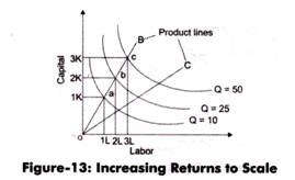
In Figure-13, a movement from a to b indicates that the amount of input is doubled. Now, the combination of inputs has reached to 2K+2L from 1K+1L. However, the output has Increased from 10 to 25 (150% increase), which is more than double. Similarly, when input changes from 2K-H2L to 3K + 3L, then output changes from 25 to 50(100% increase), which is greater than change in input. This shows increasing returns to scale.

2. Constant Returns to Scale:

The production is said to generate constant returns to scale when the proportionate change in input is equal to the proportionate change in output. For example, In Constant returns to scale, when inputs are doubled, outputs are also doubled.

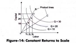
In Figure-14, when there is a movement from a to b, it indicates that input is doubled. Now, when the combination of inputs has reached to 2K+2L from IK+IL, then the output has increased from 10 to 20.

Similarly, when input changes from 2K+2L to 3K + 3L, then output changes from 20 to 30, which is equal to the change in input. This shows constant returns to scale. In constant returns to scale, inputs are divisible and production function is homogeneous.

3. Diminishing Returns to Scale:

Diminishing returns to scale refers to a situation when the proportionate change in output is less than the proportionate change in input. For example, when capital and labor is doubled but the output generated is less than doubled, the returns to scale would be termed as diminishing returns to scale.

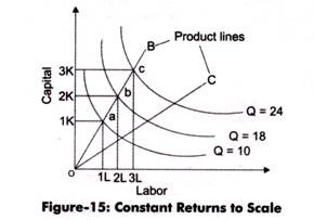
In Figure-15, when the combination of labor and capital moves from point a to point b, it indicates that input is doubled. At point a, the combination of input is 1k+1L and at point b, the combination becomes 2K+2L.

However, the output has increased from 10 to 18, which is less than change in the amount of input. Similarly, when input changes from 2K+2L to 3K + 3L, then output changes from 18 to 24, which is less than change in input. This shows the diminishing returns to scale.

Adopted from: https://www.yourarticlelibrary.com/economics/the-laws-of-returns-to-scale-production-function-with-two-variable-inputs-with-diagram/28643